

- Quickly fill up blank cells
Look at the 2-column table below, which describes the Department and Employee ID of 20 employees. However, each Department value appears only once. (This is typical of a downloaded dataset where the first column is a grouping column.)
Our task is to copy and paste the “Marketing” value from Row 3 to Row 9, “Sales” from Row 11 to 21. You might have a bigger data set, but in this case you get the idea. You can certainly drag the fill handle but imagine if you have thousands of row to fill up.
That’s where you can perform this trick. First select from cell A2 to A21, then go to Go to Home > Find & Select > Go To Special.
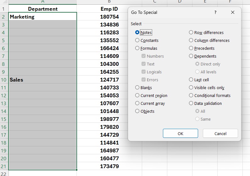
Select Blanks. (This highlights the blank cells in our table, excluding the blank rows beyond our table.)
You’ll see the cursor is in cell A3, type a =equal sign, with the up Arrow key ▲, point your cell to A2, and Marketing should be in copy mode. Once there, now instead of pressing Enter, you press Ctrl + Enter and all your cells should be filled with the correct headings.

Lastly, since you used an equal sign, Excel used it as a formula for all the cells copied, go ahead and paste the as values.
2. Show cells with Formulas
If you have a lot of formulas in your workbook or lets say, you receive a workbook from a friend or colleague and you would like to examine the formulas in that workbook. To quickly examine all the formulas go to the Formulas tab and look for Show Formulas in the Formula Auditing group. Click on it and you will be able to see the formulas, press it again to close it. Alternately, use a shortcut to open and close: Use Ctrl + Tilde (~) sign on your key pad

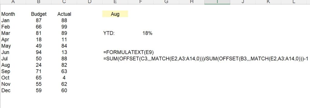
3. Use the Function FORMULATEXT
This formula will display in text format the full formula so that you can debug it and understand it in full length.
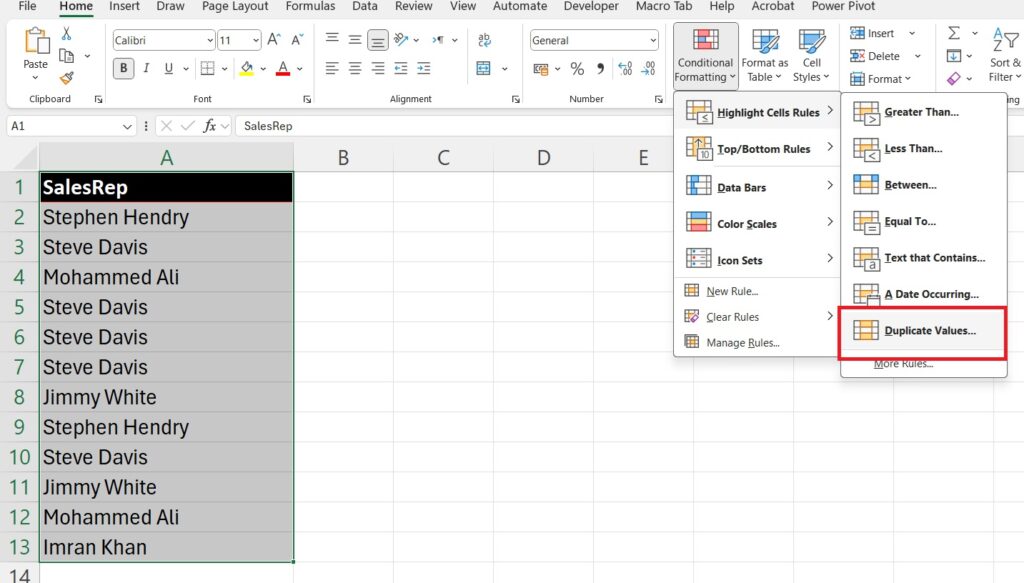
4. Quickly check for duplicates in your Data

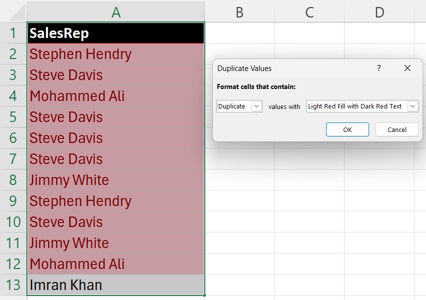
First select the data and go to Conditional Formatting from your Home tab, and click on Highlight cell rules, down below click on Duplicate Values.
The duplicate values will be highlighted in Red. Alternately you can also change from Duplicate to Unique values.
5. Activating Excel Shortcut Keys
If you click on Alt button, that activates the Shortcuts. To maneuver around the Tabs and Groups, use the highlighted Alphabets or numbers to activate that particular feature. Example: If I want to use the shortcut for bringing up the Advanced Filter Dialog box, then I use Alt + A + Q…
Using Alt + A + Q
6. Combining files from a folder using Power Query
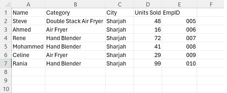
Imagine we have multiple files that we would like to combine into one Master Data. This combining process is not difficult, but it can become time-consuming and tedious and what if you later have additional data that you would like to be added into the Master Data. In this example we have 3 files inside a folder as below screen shot.

As you can see from the screen shot below the structure is same for all files, the number of columns are same, although the field headers or the columns can be in any sequence, but make sure the number of columns remain same. Data spans down the rows and can vary.

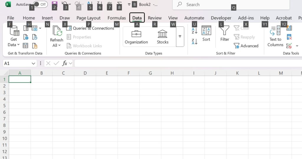
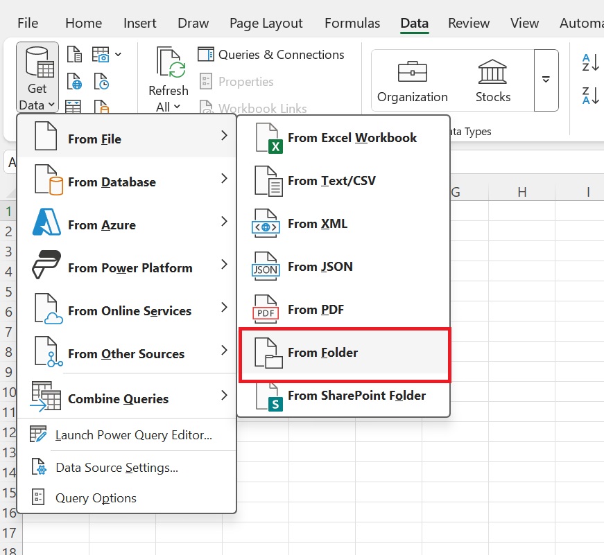
Now, lets open up a new workbook and go to the Data tab, click on Get Data which is on the extreme left side of the Ribbon. Click from File, from Folder as shown below:
Point to your folder location and click on the folder and press Open.
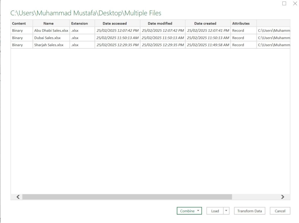
Click on Combine and Transform data from the Combine drop down list. Once done, you will come to the Combine Files dialog box, here click on Sheet1, that is the preview of your data. Click OK to continue and you will land in Power Query Editor window.
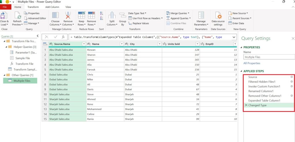
On the right hand you can see Power Query has applied steps, those steps were performed automatically. In the first column you can see all three files have been combined. You can check for the headers if they are correct. Remember that the file headers were mixed up in our files and were not in the same order. Now, you can keep the first column or delete it. Right click on column 1, where it says Source.Name and click on Remove. You will see on the right hand side that Power Query applied a new step called “Removed Columns”. Your data is now ready to load back into excel as a Master Data. Click on Close and Load To in the top left most side.
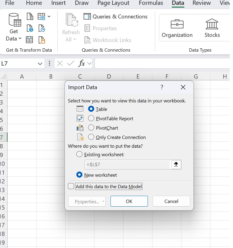
If you would like to just load the data into a table, then click ok straight away. If you want to make a Pivot table, then click on PivotTable Report and click OK.

You will see that you have successfully combined all 3 files into one Master Data. Congratulations.
The best part is that if you have another file with the same structure, then all you need to do is drop the file in that folder, go to the Pivot table and refresh and your new data will be added!
7. Knowledge of Powerful formulas like Sumif, Sumifs, Sumproduct, Subtotal, Groupby, Pivotby, Unique, Textsplit, Text, Countif.